Intro to Supervised Machine Learning (ML) Models
We will cover the following topics in this brief:
- A high-level overview of supervised machine learning
- Example: Predicting whether a point is inside a target region (Singapore islands)
- Preparing data for ML model training
- Training a Deep Neural Network (DNN) model
- Evaluating the model performance
Our objective is to gain a basic understanding of ML models and how to evaluate their performance. We will skip the mathematical details and focus on the concepts and practical applications necessary for the main lecture on Verification and Validation (V&V) for ML Models.
Supervised Machine Learning (ML)
Supervised learning is a type of ML framework where the model learns from labeled data. The model is trained on a dataset that includes input-output pairs. The goal is to learn a mapping function from input to output. The model can then predict the output for new, unseen data.
How does it differ from classical programming?
In classical programming, we write rules and logic to solve a problem. In supervised ML, we provide input-output pairs and let the model learn the rules and logic automatically. The model learns the patterns and relationships in the data to make predictions by minimizing the error between the predicted and actual labels (hence the term supervised).
How does the ML model learn the patterns in the data?
The model learns the patterns by adjusting its internal parameters based on the training data. The process is called training the model. The model is trained to minimize the error between the predicted output and the actual output. The error is measured using a loss function that quantifies the difference between the predicted and actual output.
How do we evaluate the model performance?
We evaluate the model performance using metrics such as accuracy (i.e. the percentage of correct predictions). The model is tested on a separate dataset called the test set to measure its performance on unseen data. The goal is to build a model that generalizes well to new data. To learn more about model evaluation, refer to the Evaluation Metrics.
Example: Predicting whether a point is inside a target region
Consider a simple example of predicting whether a point is inside a target region. The model learns the boundary of the target region by adjusting its parameters based on the training data. The model can then predict whether a new point is inside or outside the target region based on the learned boundary.
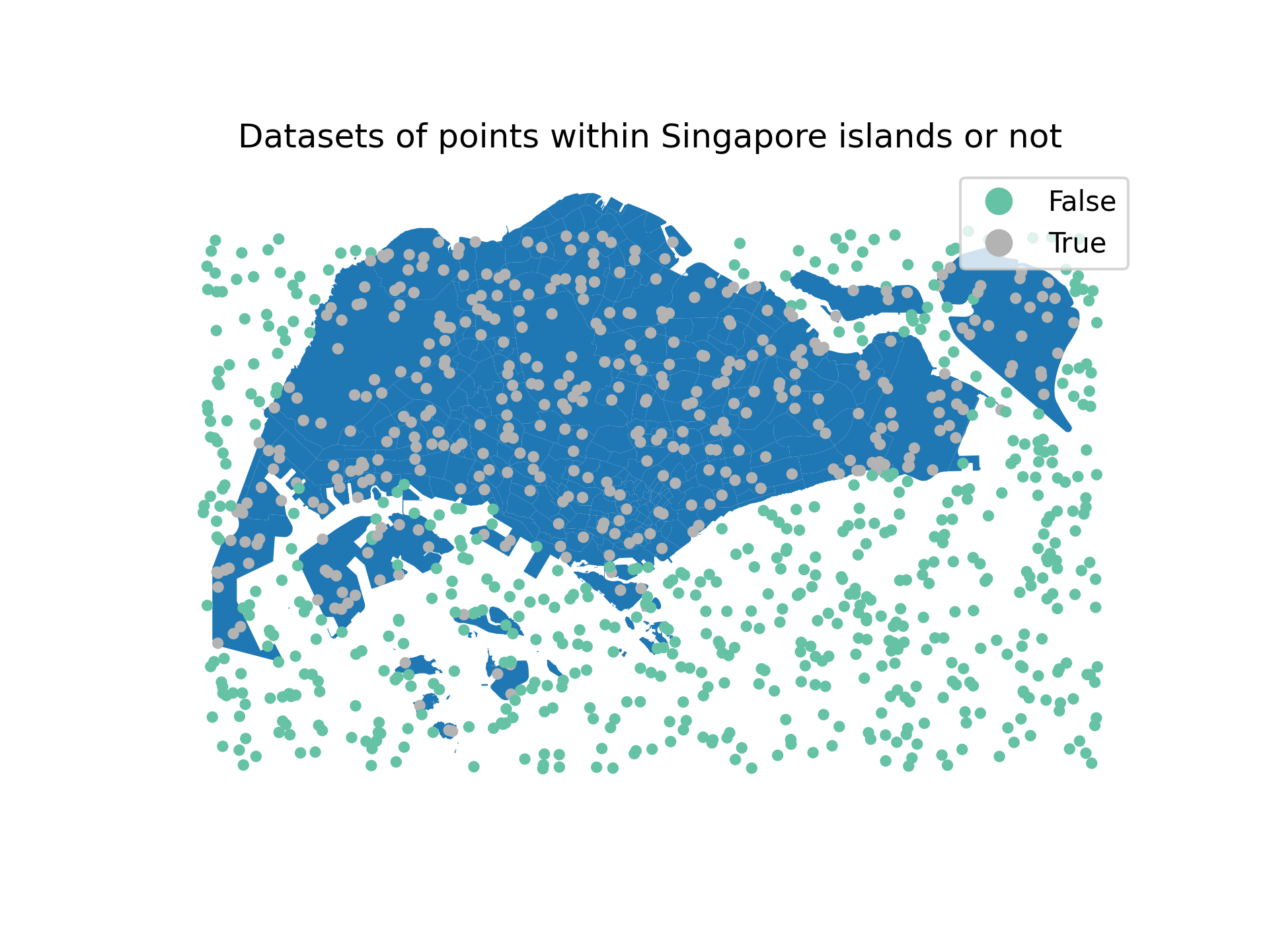
The dataset for this example is shown below.
 Fig. 1 Dataset for Predicting Point Inside Target Region (Singapore islands)
The dataset consists of points with their corresponding labels (inside or outside the islands in Singapore). Each point is a pair of coordinates (latitude, longitude) and the label is a binary value (True or False), indicating whether the point is inside the region or not. For this example, we assume to have 1500 points in the dataset.
Preparing Data for Training a ML Model
Before training the model, we need to prepare the data. For simplicity, we will use the dataset shown in Fig. 1. Suppose the dataset is stored in a dataset df with three columns: lat, lon, and label. We can split the dataset into input features X and output labels y as follows.
# Prepare the data
X = df[['lon', 'lat']].values
y = df['label'].astype(int).values
The input features X are the coordinates (longitude, latitude) and the output labels y are now binary values (0 or 1). We can then split the data into training, validation, and test sets using the train_test_split function from the sklearn library.
X_train, X_test, y_train, y_test = train_test_split(X, y, test_size=0.2, random_state=42)
X_train, X_val, y_train, y_val = train_test_split(X_train, y_train, test_size=0.2, random_state=42)
We can further preprocess the data by normalizing the input features and converting into PyTorch tensors for ease of training. Note that there are many ways to preprocess the data, even a whole field of study called Feature Engineering. See Feature Engineering for Machine Learning for more details.
# Standardize features
scaler = StandardScaler()
X_train_scaled = scaler.fit_transform(X_train)
X_val_scaled = scaler.transform(X_val)
X_test_scaled = scaler.transform(X_test)

# Convert to PyTorch tensors
X_train_tensor = torch.FloatTensor(X_train_scaled)
y_train_tensor = torch.FloatTensor(y_train)
X_val_tensor = torch.FloatTensor(X_val_scaled)
y_val_tensor = torch.FloatTensor(y_val)
X_test_tensor = torch.FloatTensor(X_test_scaled)
y_test_tensor = torch.FloatTensor(y_test)
Classification Examples using Deep Neural Networks
We will use a simple Deep Neural Network (DNN) model for classification. The model consists of an input layer, hidden layers, and an output layer. We will use the torch.nn module to define a simple DNN model.
# Define the neural network
class Net(nn.Module):
    def __init__(self):
        super(Net, self).__init__()
        self.fc1 = nn.Linear(2, 128)
        self.fc2 = nn.Linear(128, 256)
        self.fc3 = nn.Linear(256, 128)
        self.fc4 = nn.Linear(128, 64)
        self.fc5 = nn.Linear(64, 32)
        self.fc6 = nn.Linear(32, 1)

    def forward(self, x):
        x = torch.relu(self.fc1(x))
        x = torch.relu(self.fc2(x))
        x = torch.relu(self.fc3(x))
        x = torch.relu(self.fc4(x))
        x = torch.relu(self.fc5(x))
        x = torch.sigmoid(self.fc6(x))
        return x
In this example, we define a simple DNN model with 6 fully connected layers. The input layer has 2 neurons (corresponding to the latitude and longitude features) and the output layer has 1 neuron (for binary classification). The model has multiple hidden layers with ReLU activation functions and a sigmoid activation function in the output layer.
 Fig. 2 Deep Neural Network Architecture
The total number of parameters in the model is calculated as follows:
total_params = sum(p.numel() for p in model.parameters() if p.requires_grad)
print(f'Total trainable parameters: {total_params}')
# >> Total trainable parameters: 76673
We can then train the model using the training data and evaluate its performance on the validation set. We will use the torch.optim module to define an optimizer and the torch.nn.BCELoss function to define the loss function. This loss function is suitable for binary classification tasks, where the output is represented as a probability between 0 and 1. The final prediction is made by rounding the output to the nearest integer (0 or 1). See Binary Cross Entropy Loss for more details or explore Loss Functions documentation.
We will use the Adam optimizer, which is an adaptive learning rate optimization algorithm. The optimizer adjusts the learning rate during training to improve model performance. See Adam: A Method for Stochastic Optimization for more details.
model = Net()
criterion = nn.BCELoss()
optimizer = optim.Adam(model.parameters())
We can then train the model using the training data and evaluate its performance on the validation set.
# Training loop
num_epochs = 5000
for epoch in range(num_epochs):
    model.train()
    optimizer.zero_grad()
    outputs = model(X_train_tensor)
    loss = criterion(outputs.squeeze(), y_train_tensor)
    loss.backward()
    optimizer.step()

    # Validation
    model.eval()
    with torch.no_grad():
        val_outputs = model(X_val_tensor)
        val_loss = criterion(val_outputs.squeeze(), y_val_tensor)

    if (epoch + 1) % 10 == 0:
        print(f'Epoch [{epoch+1}/{num_epochs}], Train Loss: {loss.item():.4f}, Val Loss: {val_loss.item():.4f}')
Running this code will trigger iterations of training and validation. The model will adjust its parameters to minimize the loss function. The loss values will be printed at regular intervals to monitor the training progress. The training will continue for a specified number of epochs (e.g., 5000 epochs).
Epoch [10/5000], Train Loss: 0.6167, Val Loss: 0.6161
Epoch [20/5000], Train Loss: 0.4324, Val Loss: 0.4780
Epoch [30/5000], Train Loss: 0.3926, Val Loss: 0.4635
Epoch [40/5000], Train Loss: 0.3586, Val Loss: 0.4290
Epoch [50/5000], Train Loss: 0.3011, Val Loss: 0.3634
...
Epoch [4970/5000], Train Loss: 0.0082, Val Loss: 0.3869
Epoch [4980/5000], Train Loss: 0.0081, Val Loss: 0.3869
Epoch [4990/5000], Train Loss: 0.0080, Val Loss: 0.3901
Epoch [5000/5000], Train Loss: 0.0080, Val Loss: 0.3907
Evaluating the Model Performance
After training the model, we can evaluate its performance on the test set. We can calculate the accuracy of the model on the test set by comparing the predicted labels with the actual labels.
# Evaluate on test set
model.eval()
with torch.no_grad():
    test_outputs = model(X_test_tensor)
    test_loss = criterion(test_outputs.squeeze(), y_test_tensor)
    test_predictions = (test_outputs.squeeze() > 0.5).float()
    accuracy = (test_predictions == y_test_tensor).float().mean()

print(f'Test Loss: {test_loss.item():.4f}, Test Accuracy: {accuracy.item():.4f}')
# >> Test Loss: 0.9754, Test Accuracy: 0.9250
Note here that the accuracy is calculated as the percentage of correct predictions on the test set. The test loss is calculated using the same loss function as in the training and validation steps. The model’s performance can be further evaluated using other metrics such as precision, recall, F1-score, etc. See Classification Metrics for more details.
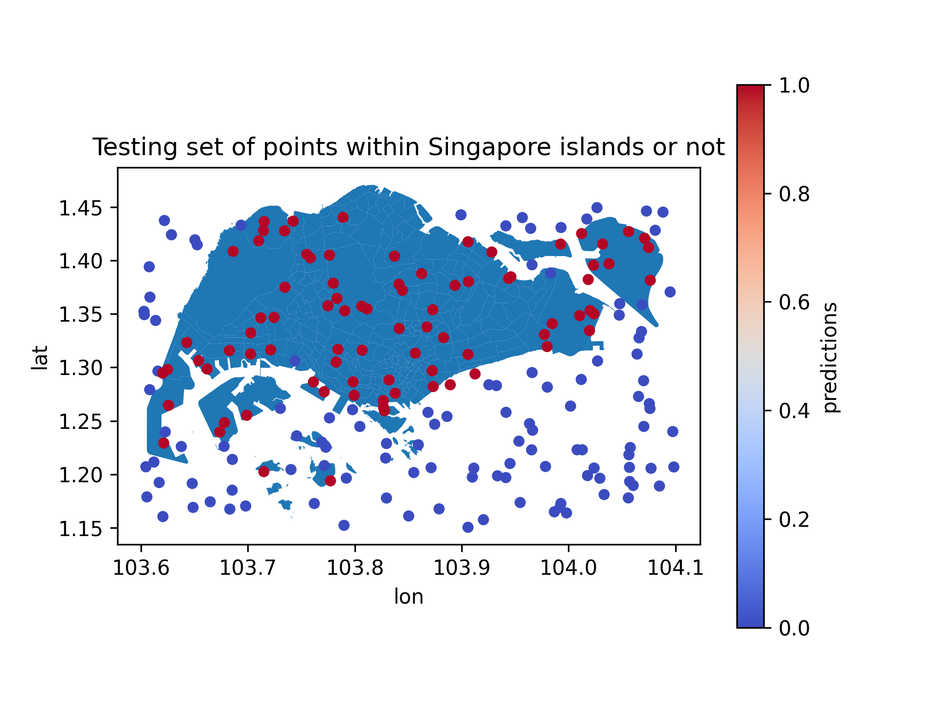
We can visualize the predicted labels on the test set to see how well the model performs in classifying points inside and outside the target region.
 Fig. 3 Predicted Labels on Test Set
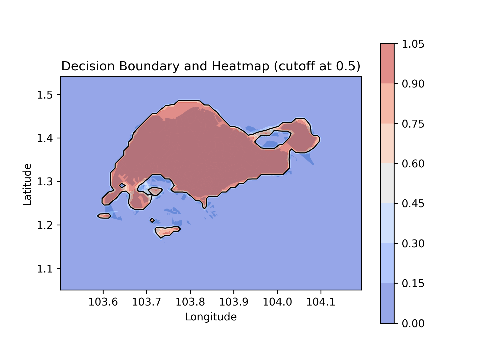
In fact, we can visualize the decision boundary learned by the model to separate the points inside and outside the target region. The decision boundary is the line that separates the two classes in the input/feature space.
 Fig. 4 Decision Boundary
To make predictions on new, unseen data, the model simply calculate the output based on the learned parameters and the input features and if the output is greater than 0.5, the model predicts the point is inside the target region, otherwise outside.
Summary
In this brief, we covered the following topics:
-
A high-level overview of supervised machine learning: Supervised learning is a type of ML framework where the model learns from labeled data. The model is trained on a dataset that includes input-output pairs to learn a mapping function from input to output. We do not need to write rules and logic explicitly as in classical programming. Instead, we provide input-output pairs and let the model learn the patterns and relationships in the data.
-
Example: Predicting whether a point is inside a target region: We used a simple example of predicting whether a point is inside a target region. The model learns the boundary of the target region based on the training data and can predict whether a new point is inside or outside the target region.
-
Preparing data for supervised machine learning: We discussed how to prepare the data for training a ML model, including splitting the dataset into input features and output labels, normalizing the input features, and converting the data into PyTorch tensors.
-
Classification examples using Deep Neural Networks: We defined a simple Deep Neural Network (DNN) model for classification and trained the model using the training data. We used the Adam optimizer and Binary Cross Entropy Loss function to train the model and evaluated its performance on the test set.
-
Evaluating the model performance: We evaluated the model performance on the test set by calculating the accuracy of the model and visualizing the predicted labels. We also visualized the decision boundary learned by the model to separate the points inside and outside the target region.
Acknowledgements
This lecture material is prepared by the instructor using various online resources and textbooks on machine learning and deep learning. The figures are created by the instructor using Subzone Census 2010 data with the help of GeoPandas and Matplotlib. The figures are rendered using Jupyter Notebook and Google Colab. The instructor acknowledges the contributions of the original authors and sources in compiling this material.
Copilot has been used to generate the text snippets and terminologies based on the input provided by the instructor. Gemini has been used within Google Colab to generate the code snippets based on the input provided by the instructor. The final content has been reviewed and edited by the instructor.
This brief is provided as a pre-reading material for the lecture on Verification and Validation (V&V) for Machine Learning (ML) Models by Mansur M. Arief. For more information, please contact the instructor directly.
Content available online at VandVAIProducts.github.io/intro-to-supervised-ml.